Guidelines on Data Visualization
In this page, the general functionality implemented in the bnviewer program is
described in detail. This covers methods that a user can visualize almost all kinds of
diffusion MRI data.
Except those specially noticed, all the data should be formatted in either NIFTI or ANAYLYZE image. NIFTI format is recommended, see Data Format page for more details.
Command Line Interface
Typing bnviewer -h in command line would given following information, which
help users to load a list of files without click them one by one.
The can be extremely useful when one wants to contantly load a large list of data files
to get screen capture images.
basic uage:
  bnviewer [[-volume] DTI_FA.nii.gz]
           [-roi ROI/roi_cc_top.nii.gz]
           [-fiber ROI/roi_cc_top.fiber]
           [-tensor DTI.nii.gz]/[-odf HARDI.nii.gz]
           [-atlas DTI.nii.gz]

options:
  -help                  show this help
  -volume  .nii.gz       set input background data
  -roi     .nii.gz       set input ROI data
  -fiber   .fiber/.trk   set input fiber data
  -tensor  .nii.gz       set input DTI data (conflict with -odf args)
  -odf     .nii.gz       set input ODF/FOD data (conflict with -tensor args)
Todo
create interface for generating high quality images and save them into specified location.
Image Data Navigation
3D Navigation
When an image data is loaded, one can change view angle by dragging left mouse button. This is the default interactor style implemented in vtkInteractorStyleTrackballCamera, which is used internally in our program. According to VTK’s documentation:
vtkInteractorStyleTrackballCamera allows the user to interactively manipulate (rotate, pan, etc.) the camera, the viewpoint of the scene. In trackball interaction, the magnitude of the mouse motion is proportional to the camera motion associated with a particular mouse binding. For example, small left-button motions cause small changes in the rotation of the camera around its focal point. For a 3-button mouse, the left button is for rotation, the right button for zooming, the middle button for panning (translation), and ctrl + left button for spinning. (With fewer mouse buttons, ctrl + shift + left button is for zooming, and shift + left button is for panning.)
We simplify the trackball interaction to used middle button for both panning and zooming, in order to spare right mouse click to popup option menu for more actions.
The background color for 3D view is defined as black by default. This can be changed from context menu popped up when right mouse click event is captured. By selecting the color from the popup color dialog, the background color is changed instantly.
Also, saving screenshots as PNG image is enabled from the context menu. The default image is named after current timestamp to avoid naming duplication.
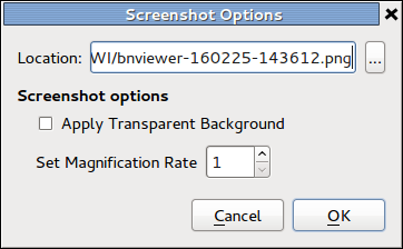
To customize generated image for different requirements, two additional options are provided, as shown in the above screenshot. The higher magnification value indicate higher resolution of generated image. By enabling transparent background in output image, one can alternate the background color in a later stage.
2D Navigation
Three 2D slice image views are placed below 3D view by default. The three slice views from left to right are sagittal plane, coronal plane and axial plane respectively.
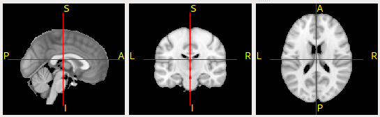
sagittal plane, coronal plane and axial plane (left to right)
2D slice view widget sizes can be enlarged by switching the overall layout. This functionality is implemented in a single button, named Switch Layout, available on the toolbar. By toggling the button, the main view panels switches between 3D view port and a combination of sliced 2d views.
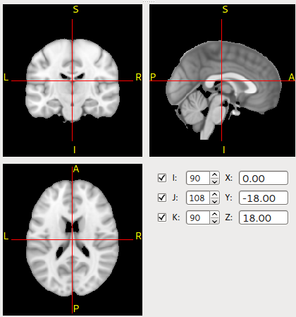
Image slice index can be changed by clicking on 2d image slice views. Besides, we perform radiological/neurological (or RAS/LAS) conversion intantly when slice index values are changed.
For people interested in more details about the radiological/neurological conversion, please refer to FSL’s Orientation Explained .
Background Volume Data Layer
Beginning from this section, several kinds of ‘layers’ are described. Each ‘layer’ may be contrain one or more data that holds the same property. By default, the layers manager is located at top-right side of the window.
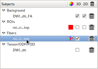
The layers manager
We refer to Background data as plain 3D or 4D volume data that user wants to visualize its sliced views. The content should be either a typical 3D image (e.g. T1/T2 image) or a 4D image such as DWI, DTI, ODF and even fMRI data.
To load a Background Data, click Load Background in the menu or toolbar, and select a single volume image. Note that selecting multiple image is not valid here, because the program doesn’t aware which background image is laid that the bottom that might be overlaid by subsequently loaded images.
Once background image is loaded, several basic data information is shown in the data property panel.
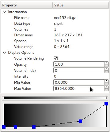
property panel showing mni152 as background image
The widget below the data property panel is the color table for Volume Rendering. The horizontal axis indicates intensity values of a target image, while the vertical axis of the widget indicate the opacity value that maps the intensity values onto visible planes in volume rendering. One can adjust opacity map (by dragging blue opacity nodes) as well as color map to get proper renderering results.
Image Contrast Enhancement
During loading a Background image, the minimum and maximum intensity values are calculated and displayed in the data property panel. By narrow down the range of image intensity values, one can the enhance image contrast.
Note that this functionality is currently applied for 2d sliced views only.
Volume Image Overlay
By loading multiple image throught Load Background menu, one can place one image over another, Therefore, it’s easy to make slice-to-slice comparison to find out image registration errors by adjusting opacity values of the upper level image.
This feature can be quite useful for verifying Skull Stripping results. After performing skull stripping, …
Todo
PUT OVERLAY IMAGE HERE!
Volume Rendering
Volume rendering of the background image can be enabled in Data Property panel. Once volume rendering is enabled, a color table is shown to enable users to adjust color map and opacity values that maps intensity values onto visible planes. This functionality is particularly useful for visualizing skull-stripped T1 image, where the folds that increase the surface area of the cortex can be directly visible without threshold-based surface extraction.
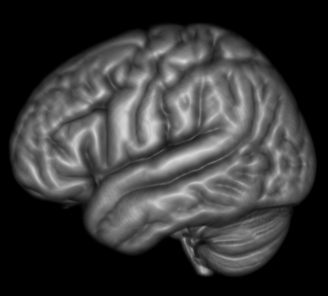
volume rendering of mni152 data
Region of Interest (ROI) Layer
To describe the location of a specific region, we employ the ROI layer. It outlines surface of the region on 3d view, along with a filled area on 2d slice views.
To open a ROI file, click on ‘Load ROI’ from either menu or toolbar. Note that loading multiple ROI data files that located within the same directory is allowed. Therefore, one don’t have load splitted brain atlas files one-by-one.
To change the color of a selected ROI files, set Color to different value from the data properties panel. This is useful when more than one ROI file is loaded, and it’s hard to distinguish them by appearance.
To adjust transparency of the surface or the filled area in 2d views, set opacity value of the selected fiber file to a value range form 0 to 1.
Todo
compute the voxel-level volume size of a region, as well as its size in millimeters (by multiplying spacing).
Fiber Layer
To display deterministic tractography results, the program generates and displays .fiber/.trk files in either lines or tubes. One can load fiber files by selecting Load Fiber either from menu or toolbar. The definition of .fiber files is available at Data Format page. The specification of .trk file format is available at TrackVis.
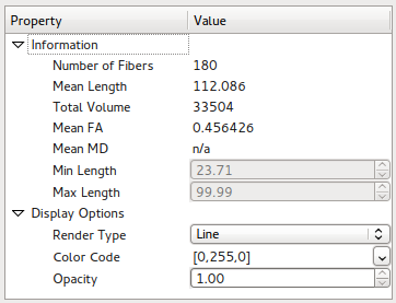
Fiber data properties panel
Basic fiber data statistics is available on data properties panel once an arbitary tract file is loaded. The statistics information include number of fibers in a tract, average length of fibers and total volume covered by the tract etc. These information are generated during fiber tracking process, and there is extra computation during online visualization.
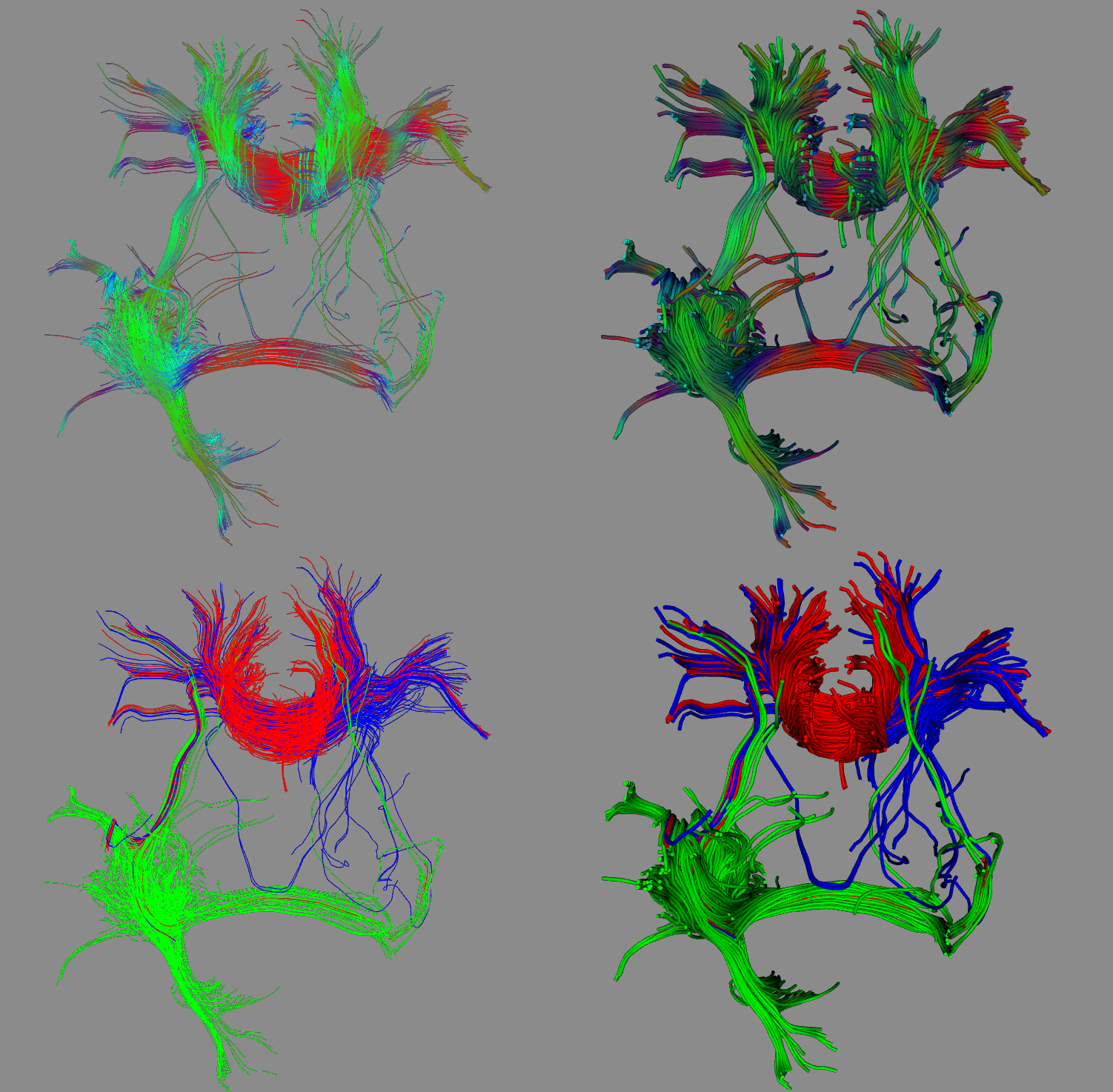
A comparison of fibers rendered in different render types.
Several display options are available to provided high quality rendering results. For performance reasons, tracts are rendered as slim lines by default. Therefore, detail shapes of the fibers are not clearly visible. However, location and orientation information of the lines are quite clear. By adjusting Color Code and Render Type, one can easily visualize multiple fiber files. On the above figure, two images on the left are fibers rendered as lines, while the two images on the right are rendered as tubes. Images on the top row are fibers rendered with directional coloring, while fibers on the bottom row are signed to a single color.
Note
Note that rendering whole brain fiber in ‘Tube’ rendering type can be quite slow for low performance computers. However, a progress bar would popup to show the current loading progress. Also, we recommand storing whole brain fiber files as .trk format instead of .fiber file to increase file loading efficiency.
Tensor/ODF/FOD Layer
Both diffusion tensor and ODF can be visualized within this layer. After adjusting rendering parameters, the Render button should be pressed in order to regenerate the scene. This prevents the time-consuming processing, every time when users are trying to change the configuration.
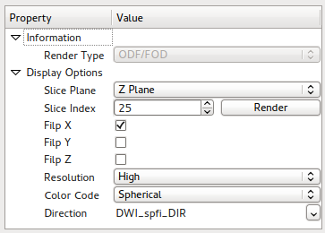
Tensor/ODF/FOD data properties panel
Diffusion tensor (DTI) file input should be a typical 4D NIFTI image, with exactly six volumes. The six values on each voxel represents entries in a 3x3 symmetric positive definite matrix. Numerical definition can be found at DTI Reconstruction section.
Diffusion orientation distribution function (ODF) file input should be a 4d image, too. However, it’s fourth dimension should be one of 15,28,45,66,91 etc. If the format is incorrect, the program would refuse to load the image to avoid potential errors. Numerical definition can be found at SPFI Reconstruction and CSD Reconstruction section.
Due to performance reasons, ODF/FOD is rendered in low resolution by default. For researchers who need high-resolution images for publication quality results, an option in the properties panel is provided.
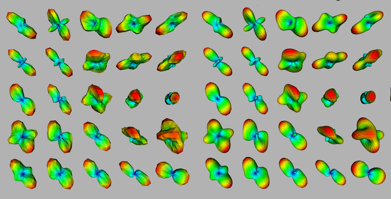
A comparison of low/high resolution ODF rendering